Lab 6-3: Bayes’ Theorem with Probability Distributions#
Example Problem of Student Quiz Scores#
In this example we are trying to figure out the probability of an event occcuring, the probability of a student getting a question right on a quiz. (Note: this problem is designed to help you answer homework 6’s problem about flooding in New York City. In the homework, you will try to figure out the probability of a flood occuring in a given year.)
Background Info for the problem:#
A student correctly answers 5 out 10 questions on the first exam in a class. On the second exam, the student correctly answers 8 of 10 questions.
From past experience, students in the class on average answer 85% of questions correctly with a standard deviation of 10%. We can assume this is normally distributed.
What fraction of the questions will the student likely answer correctly in the long run?
How does this estimate change with each exam?
import numpy as np
import scipy.stats as stats
from scipy.interpolate import interp1d
import matplotlib.pyplot as plt

%matplotlib inline
Our Bayes’ Theorem equation is:
\(P(A|B) = \displaystyle\frac{P(B|A) \cdot P(A)}{P(B)}\)
Create our prior PDF, \(P(A)\), knowing that students typically get 85% on exams, with a standard deviation of 10%.
# Our prior assumption of mean student frequency of correct answer must be between 0 and 1 (85% average test score)
mu = 0.85
# Our prior assumption of standard deviation of student scores (10% standard deviation of test score)
sigma = 0.1
# create x values over which to calculate the distribution (we'll just work in whole percentage points here)
# (x evenly spaced with 101 values between 0 and 1 (inclusive))
x = np.linspace(0, 1, 101)
# Bayesian prior distribution based on past students (normalized so that the area under the curve = 1)
pdf = stats.norm.pdf(x, mu, sigma)

# this is the pdf of P(A)
prior_pdf = pdf / np.sum(pdf)
# and the cdf
prior_cdf = np.cumsum(prior_pdf)
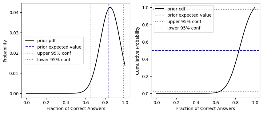
We can find the expected test score value by multiplying the prior_pdf by the test score values (x):
prior_expected = np.sum(prior_pdf * x)
print("expected value: {}".format( np.round(prior_expected,2)))
expected value: 0.84
And we can find the upper and lower 95% confidence limits using the cdf.
f = interp1d(prior_cdf, x)
upper = f(0.975)
lower = f(0.025)
print("upper: {}".format( np.round(upper,2)))
print("lower: {}".format( np.round(lower,2)))
upper: 0.98
lower: 0.65
To find the cumulative probability value that corresponds to our prior expected, we can also use the interp1d function to look it up on the cdf.
g = interp1d(x, prior_cdf)

prior_expected_cdf = g(prior_expected)
prior_expected_cdf
array(0.49927539)
Plot the prior distribution
fig, [ax1, ax2] = plt.subplots(1,2, figsize=(10,4))

ax1.plot(x,prior_pdf, 'k', label='prior pdf')
ax1.axvline(prior_expected, linestyle='--', color='b', label='prior expected value')
ax1.axvline(upper, linestyle=':', color='grey', label='upper 95% conf')
ax1.axvline(lower, linestyle=':', color='grey', label='lower 95% conf')
ax1.set_xlabel('Fraction of Correct Answers')
ax1.set_ylabel('Probability')
ax1.legend(loc='center left')

ax2.plot(x,prior_cdf, 'k', label='prior cdf')
ax2.axhline(prior_expected_cdf, linestyle='--', color='b', label='prior expected value')
ax2.axhline(0.975, linestyle=':', color='grey', label='upper 95% conf')
ax2.axhline(0.025, linestyle=':', color='grey', label='lower 95% conf')
ax2.set_xlabel('Fraction of Correct Answers')
ax2.set_ylabel('Cumulative Probability')
ax2.legend(loc='upper left')
<matplotlib.legend.Legend at 0x7f4c027aa3d0>
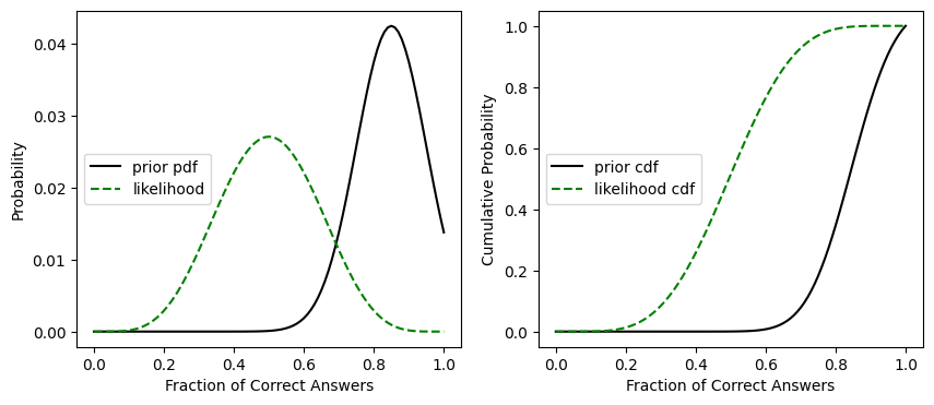
The student takes their first exam
The student gets 5 out of 10 questions right on their first exam.
Create the pdf representing the likelihood of getting this score, \(P(B|A)\). This comes from a binomial distribution.
# this is our P(B|A)
likelihood = stats.binom.pmf(5, 10, x)
We can plot this likelihood distribution on top of our prior to see what it looks like
fig, [ax1, ax2] = plt.subplots(1,2, figsize=(10,4))

ax1.plot(x,prior_pdf, 'k', label='prior pdf')
ax1.plot(x,likelihood/np.sum(likelihood), 'g--', label='likelihood') # note that I'm temporarily normalizing the likelihood PDF plot here
ax1.set_xlabel('Fraction of Correct Answers')
ax1.set_ylabel('Probability')
ax1.legend(loc='center left')

ax2.plot(x,prior_cdf, 'k', label='prior cdf')
ax2.plot(x,np.cumsum(likelihood/np.sum(likelihood)), 'g--', label='likelihood cdf') # note that I'm temporarily normalizing the likelihood CDF plot here
ax2.set_xlabel('Fraction of Correct Answers')
ax2.set_ylabel('Cumulative Probability')
ax2.legend(loc='center left')
<matplotlib.legend.Legend at 0x7f4c0238c4d0>
Multiply by our prior distribution to get \(P(B|A) \cdot P(A)\)
# this is  P(B|A)*P(A)
likelihood_prior = likelihood * prior_pdf
However, this isn’t our posterior pdf yet. We need to normalize by dividing by \(P(B)\).
And we can calculate this using the chain rule: \(P(B) = \displaystyle\sum{P(B|A_i)P(A_i)}\) which in our case is the sum of all likelihood * prior_pdf.
This finally gives us the posterior pdf, \(P(A|B)\)
# this gives us P(A|B)
post_pdf = likelihood_prior / np.nansum(likelihood_prior)
post_cdf = np.cumsum(post_pdf)
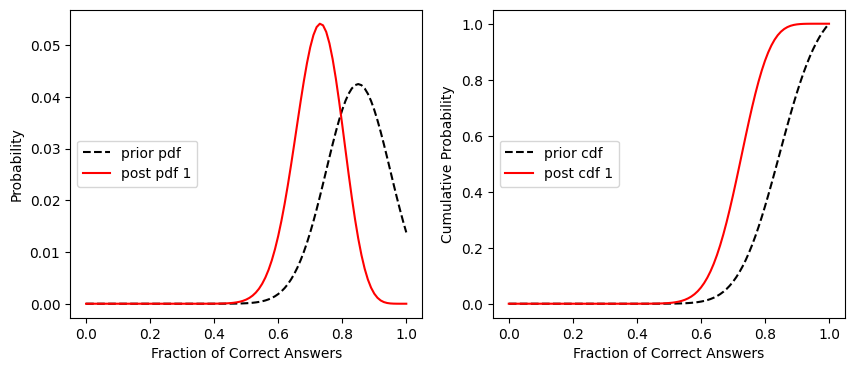
And we can compute the expected value, and upper and lower confidence intervals for 95%
post_expected = np.sum(post_pdf * x)
print("expected value: {}".format( np.round(post_expected,2)))

f = interp1d(post_cdf, x)
post_upper = f(0.975)
post_lower = f(0.025)
print("upper: {}".format( np.round(post_upper,2)))
print("lower: {}".format( np.round(post_lower,2)))
expected value: 0.72
upper: 0.85
lower: 0.57
Plot the prior pdf and posterior pdf
fig, [ax1, ax2] = plt.subplots(1,2, figsize=(10,4))

ax1.plot(x,prior_pdf, '--k', label='prior pdf')
ax1.plot(x,post_pdf, 'r', label='post pdf 1')
ax1.set_xlabel('Fraction of Correct Answers')
ax1.set_ylabel('Probability')
ax1.legend(loc='center left')


ax2.plot(x,prior_cdf, '--k', label='prior cdf')
ax2.plot(x,post_cdf, 'r', label='post cdf 1')
ax2.set_xlabel('Fraction of Correct Answers')
ax2.set_ylabel('Cumulative Probability')
ax2.legend(loc='center left')
<matplotlib.legend.Legend at 0x7f4c02287bd0>
The student takes their second exam
For the next iteration of Bayes’ Theorem, we use the posterior pdf as our new prior pdf.
# this is the pdf of P(A), which was our posterior above, P(A|B)
prior_pdf2 = post_pdf.copy()
# and the cdf
prior_cdf2 = np.cumsum(prior_pdf2)
On their second exam, the student gets 8 out of 10 correct.
Create the pdf representing the likelihood of getting this score, \(P(B|A)\).
# this is our P(B|A)
likelihood2 = stats.binom.pmf(8, 10, x)
Multiply by our prior distribution to get \(P(B|A) \cdot P(A)\)
# this is  P(B|A)*P(A)
likelihood_prior2 = likelihood2 * prior_pdf2
Normalize by dividing by \(P(B)\).
And we can calculate this using the chain rule: \(P(B) = \displaystyle\sum{P(B|A_i)P(A_i)}\) which in our case is the sum of all likelihood * prior_pdf.
This finally gives us the posterior pdf, \(P(A|B)\)
# this gives us P(A|B)
post_pdf2 = likelihood_prior2 / np.nansum(likelihood_prior2)
post_cdf2 = np.cumsum(post_pdf2)
Compute the expected value, and upper and lower confidence intervals for 95%
post_expected2 = np.sum(post_pdf2 * x)
print("expected value: {}".format( np.round(post_expected2,2)))

f = interp1d(post_cdf2, x)
post_upper2 = f(0.975)
post_lower2 = f(0.025)
print("upper: {}".format( np.round(post_upper2,2)))
print("lower: {}".format( np.round(post_lower2,2)))
expected value: 0.74
upper: 0.85
lower: 0.6
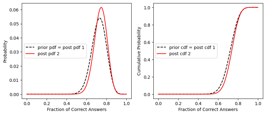
Plot the prior pdf and posterior pdf
fig, [ax1, ax2] = plt.subplots(1,2, figsize=(10,4))

ax1.plot(x,prior_pdf2, '--k', label='prior pdf = post pdf 1')
ax1.plot(x,post_pdf2, 'r', label='post pdf 2')
ax1.set_xlabel('Fraction of Correct Answers')
ax1.set_ylabel('Probability')
ax1.legend(loc='center left')

ax2.plot(x,prior_cdf2, '--k', label='prior cdf = post cdf 1')
ax2.plot(x,post_cdf2, 'r', label='post cdf 2')
ax2.set_xlabel('Fraction of Correct Answers')
ax2.set_ylabel('Cumulative Probability')
ax2.legend(loc='center left')
<matplotlib.legend.Legend at 0x7f4c01f65510>
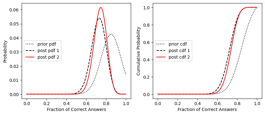
Plot the original distribution, and our two updates all together
fig, [ax1, ax2] = plt.subplots(1,2, figsize=(10,4))

ax1.plot(x,prior_pdf, ':k', label='prior pdf')
ax1.plot(x,prior_pdf2, '--k', label='post pdf 1')
ax1.plot(x,post_pdf2, 'r', label='post pdf 2')
ax1.set_xlabel('Fraction of Correct Answers')
ax1.set_ylabel('Probability')
ax1.legend(loc='center left')

ax2.plot(x,prior_cdf, ':k', label='prior cdf')
ax2.plot(x,prior_cdf2, '--k', label='post cdf 1')
ax2.plot(x,post_cdf2, 'r', label='post cdf 2')
ax2.set_xlabel('Fraction of Correct Answers')
ax2.set_ylabel('Cumulative Probability')
ax2.legend(loc='center left')
<matplotlib.legend.Legend at 0x7f4c01eedc10>
What fraction of the questions will the student likely answer correctly in the long run?
How does this estimate change with each exam?
The answer to these questions is just our expected value from the posterior pdfs after each of the two updates:
print("prior expected value: {}%".format(100*np.round(prior_expected,2)))
print("posterior expected value after 1st exam: {}%".format(100*np.round(post_expected,2)))
print("posterior expected value after 2nd exam: {}%".format(100*np.round(post_expected2,2)))
prior expected value: 84.0%
posterior expected value after 1st exam: 72.0%
posterior expected value after 2nd exam: 74.0%
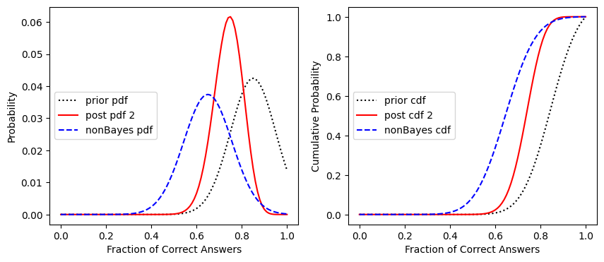
What if we had used frequentist statistics, and therefore determined the student’s expected exam value only based on their performance on the two exams so far?
The non-Bayesian sample mean and standard deviation are based on the two completed exams, using sample size of 2x10=20, where each question is considered independent.
Our expected value is then the sum of all correct answers over the sum of all questions across all exams so far: \(\bar{p} = \displaystyle\sum^m{\frac{c}{n}}=\frac{5+8}{2\times10}\)
# this is expected p (student's probability of correct answer), number of successes divided by, the number of questions per test times the number of tests
p_bar = (5+8) / (10+10)
Because each question has only two states, correct or incorrect (1 or 0), we use the standard deviation of a binomial distribution to create the PDF:
For example, over \(n\) trials, the variance of the number of successes/failures is measured by \(\sigma^2 = n\cdot p \cdot(1-p)\)
And the variance of the probability of success is the above variance divided by \(n^2\)
So \(\sigma_p= \sqrt{(\sigma^2/n^2)} = \sqrt{(p\cdot(1-p)/n)} \)
sigma_p = np.sqrt(p_bar*(1-p_bar)/(10+10))

# create the PDF
nonBayes_pdf = stats.norm.pdf(x, p_bar, sigma_p)
nonBayes_pdf = nonBayes_pdf / np.nansum(nonBayes_pdf)
# compute the CDF from a cumulative sum of the PDF
nonBayes_cdf = np.cumsum(nonBayes_pdf)
Now plot the prior pdf, the bayesian pdf after the two exams, and the non-bayesian PDF for our student who’s completed two tests so far:
fig, [ax1, ax2] = plt.subplots(1,2, figsize=(10,4))

ax1.plot(x,prior_pdf, ':k', label='prior pdf')
ax1.plot(x,post_pdf2, 'r', label='post pdf 2')
ax1.plot(x,nonBayes_pdf, '--b', label='nonBayes pdf')
ax1.set_xlabel('Fraction of Correct Answers')
ax1.set_ylabel('Probability')
ax1.legend(loc='center left')

ax2.plot(x,prior_cdf, ':k', label='prior cdf')
ax2.plot(x,post_cdf2, 'r', label='post cdf 2')
ax2.plot(x,nonBayes_cdf, '--b', label='nonBayes cdf')
ax2.set_xlabel('Fraction of Correct Answers')
ax2.set_ylabel('Cumulative Probability')
ax2.legend(loc='center left')
<matplotlib.legend.Legend at 0x7f4c01b0cf10>