Lab 5-2: Autocorrelation#
import numpy as np
import pandas as pd
import scipy.stats as stats
import scipy.io as sio # scipy input/output functions for reading a .mat file
import datetime as dt # for formatting dates and times
import matplotlib.pyplot as plt
%matplotlib inline
Load some example data of air temperature measured with iButton temperature sensors.
Unpack the mat file into numpy arrays, format dates to python datetimes following the method outlined here.
# load the ibutton data
data = sio.loadmat('../data/iButtons_2008-2010.mat')

# convert matlab format dates to python datetimes
datenums = data['TIME'][:,0]
dates = [dt.datetime.fromordinal(int(d)) + dt.timedelta(days=d%1) - dt.timedelta(days = 366) for d in datenums]
pd.plotting.register_matplotlib_converters()

# Unpack the rest of the data
SITE_NAMES = [name[0][0] for name in data['SITE_NAMES']]
SITE_LATS = data['SITE_LATS'][:,0]
SITE_LONS = data['SITE_LONS'][:,0]
SITE_ELEVS = data['SITE_ELEVS'][:,0]
AIR_TEMPERATURE = data['AIR_TEMPERATURE']
AIR_TEMPERATURE_ZEROMEAN = data['AIR_TEMPERATURE_ZEROMEAN']
nt = data['nt'][0][0] # size in the t dimension
nx = data['nx'][0][0] # size in the x dimension (number of sites)
Plot a timseries for one of the sites in our dataset
site = 3
# create a figure and specify its size
plt.figure(figsize=(10,5))

plt.plot(dates,AIR_TEMPERATURE[:,site], label=SITE_NAMES[site])

plt.legend(loc='lower left')                   # add a legend to the lower left of the figure
plt.ylabel('Air Temperature, C')               # set the label for the y axis
plt.xlabel('Time')                             # set the label for the x axis
plt.title('iButton Air Temperature');          # give our plot a title
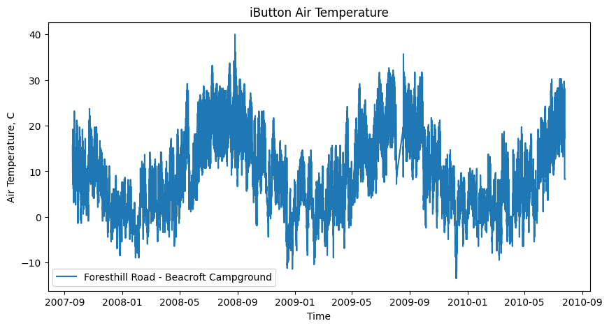
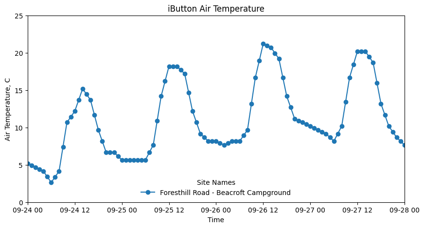
It’s hard to see what’s going on in detail, so we’ll set x and y axes limits to “zoom in” to just a few days
# create a figure and specify its size
plt.figure(figsize=(10,5))

plt.plot(dates,AIR_TEMPERATURE[:,site], '-o', label=SITE_NAMES[site])

plt.legend(frameon=False,
           loc='lower center',
           labelspacing=0.5,
           title='Site Names')                 # add a legend and format
plt.ylabel('Air Temperature, C')               # set the label for the y axis
plt.xlabel('Time')                             # set the label for the x axis
plt.title('iButton Air Temperature');          # give our plot a title

# use xlim to set x axis limits to zoom in between two specific dates
plt.xlim(('2007-09-24', '2007-09-28'));

# use ylim to set y axis limits to zoom in between two specific temperatures
plt.ylim((0,25));
Compute the autocorrelation of this dataset for different lag values
There are a few functions we could use like pandas.Series.autocorr if we have our data in a pandas dataframe, but here I’m going to use np.corrcoef():
# start with a lag of 1 hour, but then change this and run the cell a few times to try out different values
lag = 1

# our dataset of air temperatures for this site will go from the beginning all the way to n-k,
# or using python's negative indexing notation we can say it goes all the way to index -lag
x = AIR_TEMPERATURE[:-lag,site]

# create a "lagged" dataset by removin the first k numbers
y = AIR_TEMPERATURE[lag:,site]

# calculate the autocorrelation
R = np.corrcoef(x,y)
print('Autocorrelation at lag={} is R='.format(lag))
print(R)
Autocorrelation at lag=1 is R=
[[1.         0.98782022]
 [0.98782022 1.        ]]
This gives us a matrix of correlation values for the variables we input. Notice here that its symmetrical, so we can pick one to report our autocorrelation value.
print('Autocorrelation at lag={} is R={}'.format(lag, R[0][1]))
Autocorrelation at lag=1 is R=0.9878202154947485
Now loop through all lag value from k=1 to k=n/4 (it’s advised not to use lags > n/4), and save all the autocorrelation values to an array.
# make an array of our lag values that we want
lags = np.arange(1,int(len(AIR_TEMPERATURE[:,site])/4))
# create an empty array to store autocorrelation values in
R = np.empty(len(lags))
# loop through all the lags and compute autocorrelation
for i, k in enumerate(lags):
    # our dataset of air temperatures for this site will go from the beginning all the way to n-k,
    # or using python's negative indexing notation we can say it goes all the way to index -lag
    x = AIR_TEMPERATURE[:-k,site]
    # create a "lagged" dataset by removin the first k numbers
    y = AIR_TEMPERATURE[k:,site]
    # calculate the autocorrelation
    R[i] = np.corrcoef(x,y)[0][1]
Plot autocorrelation versus lag
fig, ax = plt.subplots(figsize=(10,5))

ax.plot(lags, R,'.')

ax.set_ylabel('Autocorrelation, R')
ax.set_xlabel('Lag, hours')
ax.set_title('Autocorrelation versus Lag for Air Temperature\nat {}'.format(SITE_NAMES[site]));
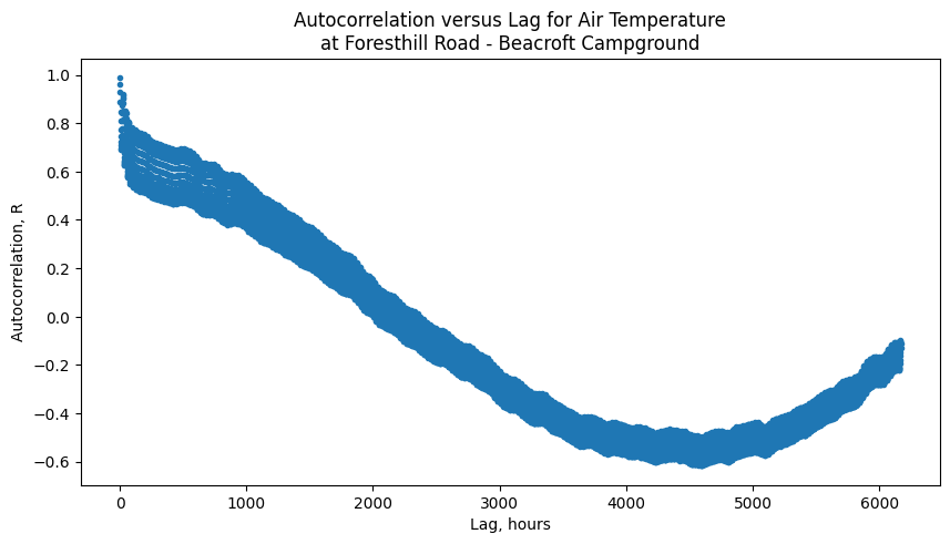
Adjust the axes limits to zoom in to the first couple hunderd lag values to see what’s going on here.
fig, ax = plt.subplots(figsize=(10,5))

ax.plot(R,'.')

ax.set_xlim((0,200))
ax.set_ylim((0,1))

ax.set_ylabel('Autocorrelation, R')
ax.set_xlabel('Lag, hours')
ax.set_title('Autocorrelation versus Lag for Air Temperature\nat {}'.format(SITE_NAMES[site]));
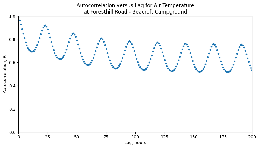
Notice the wavy pattern, it’s peaking about every 24 hours meaning that while we have our highest autocorrelation just a lag of 1 or 2 hours, we also get high autocorrelations around 24 hours, or 48 hours, or 72 hours, and every multiple of 24.