Airborne Snow Observatory, Olympic Mountains Lidar

Dec. 2017

First Return Point Density Analysis

Background Information:

A lidar instrument calculates the distance to, and the relative position of, a distant point using the return time of flight of the reflected laser and the known laser emission geometry. [6] The reflecting point’s position with respect to Earth’s surface can then be determined by using the instrument’s precise location, as informed by GPS and inertial navigation. [6] Divergenge, or spread, of a laser beam on the order of 0.3-1.0 mrad corresponds to a laser footprint size of 0.3-1.0 m at a distance of 1000 m from the target surface. This beam divergence allows a single laser pulse to reflect off of multiple objects at different heights within the footprint area. These multiple reflections are read by the instrument as a return wavepacket, which can then be discretized into a number of returns at specific points that met a return intensity threshold. [3]

The point density of a lidar dataset can be quantified as the average number of laser pulse return signals detected per unit area. Alternatively, this can also be reported as a linear measurement of the average spacing between points. Point density of lidar data acquired from an aircraft is a function of instrument parameters and aircraft motion. The instrument’s laser pulse rate, and scan rate (the oscillating or rotating mirror’s angular velocity) can provide information about the minimum cross-track point spacing. The down-track point spacing is controlled by the aircraft’s ground speed, the instrument’s scan rate, and scan pattern. The scan angles covered by the instrument, the aircraft’s altitude (AGL), and the flight line control the overlapping of ground tracks (swath width) that can greatly increase point density and help to minimize errors by scanning locations from multiple angles. [1] Point density can change at a finer scale within a single flight line as changes in aircraft pitch can cause scan line overlaps or gaps. Surfaces closer to normal with the incident laser pulse (smaller angle of incidence) can return higher intensity reflections, especially in steeply sloping terrain where “timewalk” errors can occur.

The first return point density of a lidar product provides information about how the data can be used in further analysis, and if special considerations need to be made in areas of greatly differing point density. Many applications utilizing lidar data rely on creating a digital surface model (DSM) from the collected point cloud (such as in the case of determining snow depth by subtracting snow-off from snow-on DSMs). These DSM are created by methods of interpolation (such as inverse distance weighting, IDW) between observed points. The resulting DSM grid element size should match the magnitude of the average point spacing (a measure of point density). Performing interpolation with low point density data can lead to a smoother DSM and the loss of sub-grid features. [1]

Errors in measured lidar points can be introduced from the instrument itself, complex or sloping terrain, thick vegetation, and absorptive or scattering surfaces. Instrument/aircraft position errors from the GPS/INS (< 0.1 m) are of smaller magnitude than external error sources (0.1 - 0.5 m). [5] Steeply sloping terrain can induce apparent errors in the Z (height) direction when errors (from other sources) occur in X and/or Y. Similarly, “timewalk” errors occur when a diverged laser beam reflects off a steep slope, causing a delay in the return time of the wavepacket intensity threshold for a discrete return, and an over-estimate in the distance to the measured point. Minimizing the number of laser pulses with large incidence angles (such as nadir pulses onto steep slopes) can help avoid these types of errors (which can be on the order of 0.5 m). Thick vegetation can make determining the ground surface beneath the vegetation more difficult and introduce errors on the order of 0.1 m. Regarding the measurement of surfaces coated in snow and ice, changes in grain size can alter the returned wavepacket intensity, and can introduce further errors. [1]

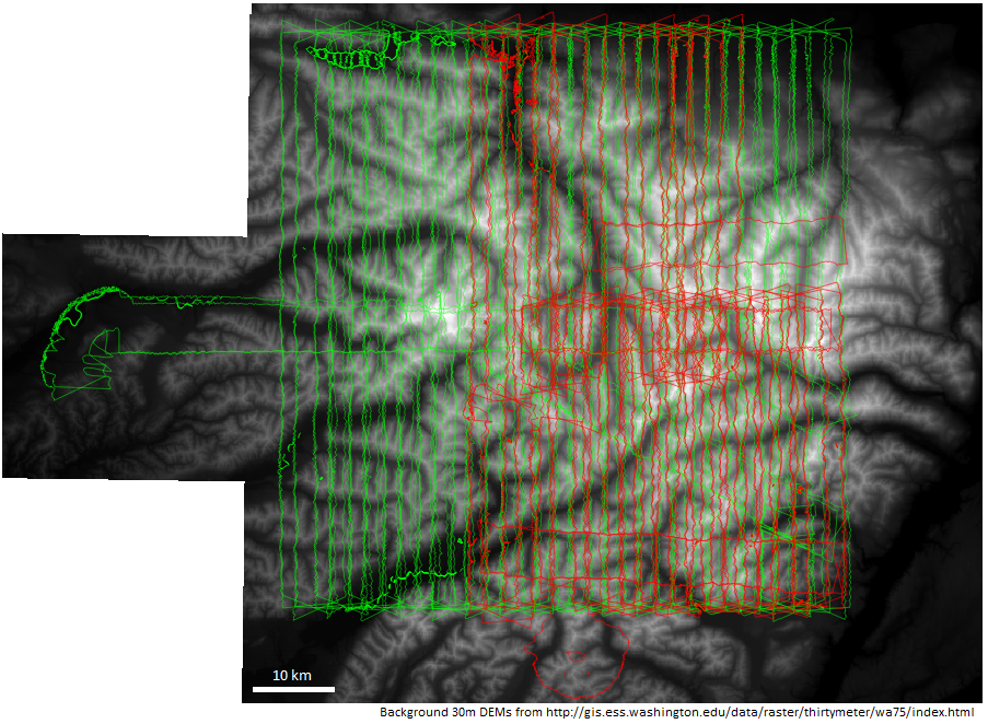
JPL’s Airborne Snow Observatory (ASO) conducted a series of flights over the Olympic Mountains in 2015-2016 to collect lidar and spectrometer data in snow-off and snow-on conditions.[2] Point density maps were created for LAS files from the ASO flights on February 8, 9, and March 29, 30 in 2016.

Olympics Snow-On Lidar Coverage

red = Feb. 8,9 2016

green = Mar. 29, 30 2016

Footprints produced using QGIS Plugin: Image Footprint

The candidate requirements for these flights were to obtain lidar data with a Nominal Point Spacing (NPS), of 0.3 m, or 12 points/m^2, a Ground NPS of 0.5, or 4 points/m^2, and a beam divergence < 0.5 mrad. The instrument operated with a laser wavelength of 1064 nm, in the near infrared (NIR), and an 800 MHz pulse rate. This wavelength provides high snow reflectance and minimal penetration into the snow to accurately measure the snow surface. [3] The LAS files processed by the ASO team from the raw flight data have filtered discrete returns from the full measured return wavepacket (where the wavepacket intensity exceeded a certain threshold). [4] Each LAS file contains the data collected in a single aircraft flightline, and was processed individually to produce a point density map.

First Return Point Density Workflow:

Each LAS file was processed using a PDAL pipeline to select only the first return detected from each laser pulse emitted. Only the first returns were considered in these point density maps in order to remove some of the factors that beam divergence, vegetation and other sub-footprint surface variations would have on reporting point density from all returns. When all returns are considered, the point density also shows surface “roughness” rather than factors of interest here such as beam incident angle and aircraft position and flight path. These first returns were then binned into 10m pixels and written out as a raster. The values of these pixels report the number of first returns received from within the 10x10m pixel ( pts/10m^2), which can be converted to the standard point density measure of pts/m^2. A batch file was written to process whole directories of LAS files through the PDAL pipeline. Within a GIS package (QGIS was used here) these rasters can be added together to compute the final point density within each pixel that resulted from overlaps in flightline swaths.

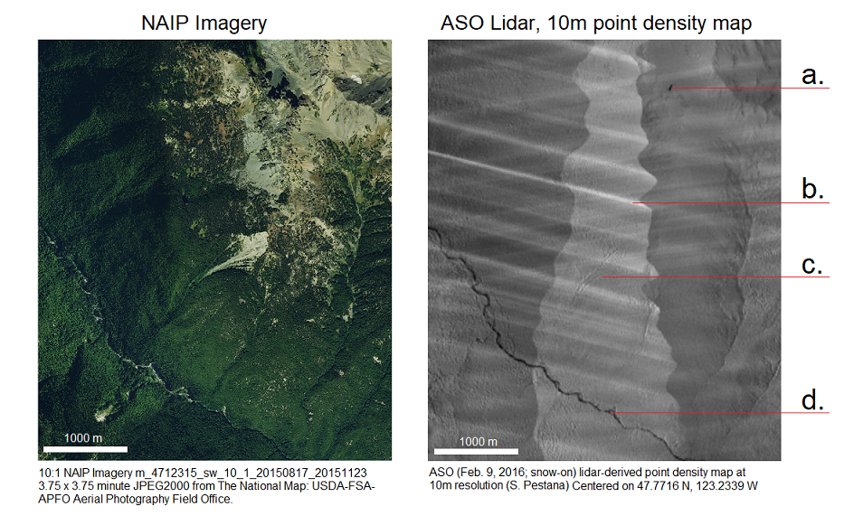
First Return Point Density Example

a. Lidar “shadow” between steep rock outcrops with very low first return point density ( < 0.1 pts/m^2) (Little Mystery, Mount Mystery)

b. Bright (higher first return point density) band possibly from slight change in aircraft speed or pitch causing scan line overlaps ( > 2 pts/m^2)

c. Region within flight line overlaps shows a higher overall average first return point density ( ~1 pts/m^2)

d. Low first return point density nearest to river surface (Dosewallips River) ( 0-0.1 pts/m^2)

First Return Point Density Pipeline (first_return_point_density.json)

Input and output filepaths are substituted in batch run
Using filters.range to select first returns:
- limits - selecting only the first returns (range from 1 to 1)
Using writers.gdal to write out raster image
- resolution - pixel side length in units of original las file (use lasinfo or pdal info to get file metadata and statistics)
- output_type - “count” for number of points within each pixel (other options)
- gdaldriver - GeoTiff

{
  "pipeline":[
	"input.las",
    {	
	  "tag" : "firstReturns",
      "type" : "filters.range",
      "limits" : "ReturnNumber[1:1]"
    },
    {
	  "tag" : "densityRaster",
      "type" : "writers.gdal",
	  "inputs" : [
					"firstReturns"
				 ],
	  "resolution": 10,
	  "output_type" : "count",
	  "gdaldriver" : "GTiff",
      "filename" : "output.tif"
    }
  ]
}

Batch Script (point_density.bat)

Find files to process: (CAUTION - All files matching LASdir and LASext will be processed)
- LASdir - set to directory containing files to process
- LASext - file extention (.las or .laz) to identify files to process in LASdir
PIPELINE - point to .json pipeline file to run each .las file through
Change output filename by editing the line ` –writers.gdal.filename=”G:\%%~nf_xxxxxx.tif”`
Run

@echo off
setlocal
set "LASdir=C:\lasfiles_to_process"
set "PIPELINE=C:\pdal-pipelines\first_return_point_density.json"
set "LASext=las"
pushd %LASdir%
for /R %LASdir% %%f in (*.%LASext%) do (
echo %%f
pdal pipeline "%PIPELINE%"^
 --readers.las.filename="%%f"^
 --writers.gdal.filename="G:\%%~nf_1STreturn_pointDensity_10m.tif"
)
endlocal

[1] Deems, Painter. Lidar Measurement of Snow Depth: Accuracy and Error Sources, 2006. Montana State University Library

[2] Houze, et al. The Olympic Mountains Experiment (OLYMPEX) Oct 2017. Bulletin of the American Meteorological Society. Vol 98-10

[3] Deems. “Lidar Altimetry: Parameters & requirements development for SnowEx” March 2016. NASA SnowEx Planning Meeting.

[4] Deems, Painter, ASO Team. “NASA ASO: Measuring Spatial Distribution of Snow Water Equivalent and Snow Albedo” Aug 2015. ASO UT Snow Workshop Presentation.

[5] Deems, Painter, Finnegan. Lidar measurement of snow depth: a review Jul 2013. Journal of Glaciology. Vol 59-215. pp 467-479

[6] National Oceanic and Atmospheric Administration (NOAA) Coastal Services Center. 2012. “Lidar 101: An Introduction to Lidar Technology, Data, and Applications.” Revised. Charleston, SC: NOAA Coastal Services Center.

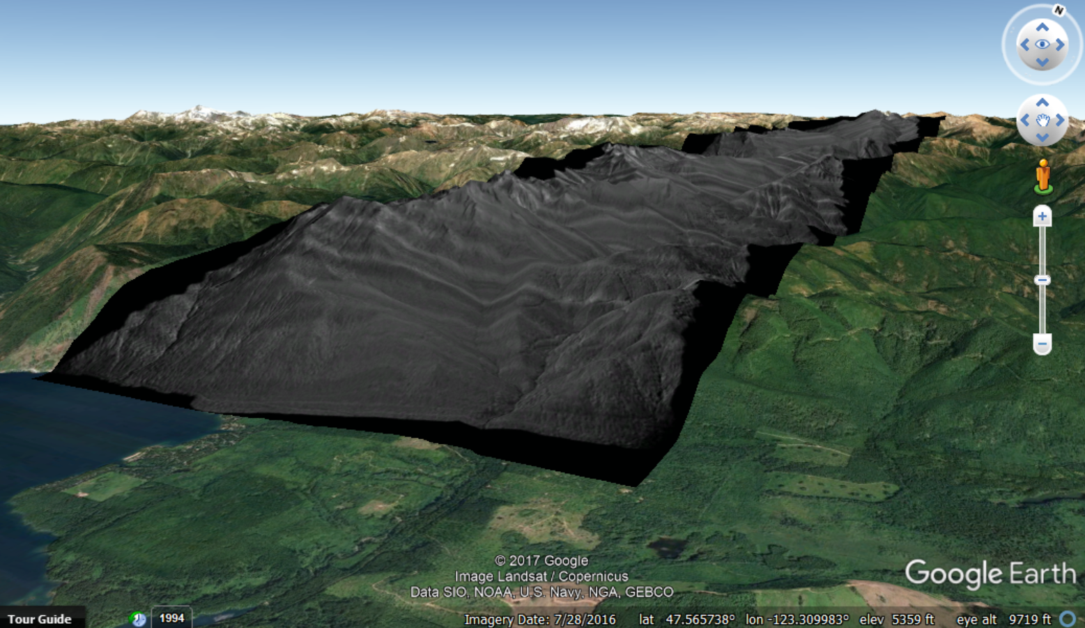
Google Earth Overlay Example

Notes on PDAL Pipelines

Processing lidar data with PDAL - Point Data Abstraction Library

Splitting LAS Files

Specify input filepath
Use filters.divider with the following options:
- mode - “partition” (default) or “round_robin” processing
- count - Provide number of output files to create from single input
- capacity - Alternatively, provide the number of points to be contained in each output file
Use writers.las to write out new las files
- filename - include “#” character in output filename for incremental numbering of split files

{
  "pipeline":[
    "\input\filepath\filename.las",
    {
      "tag" : "splitLasFile",
      "type" : "filters.divider",
      "mode" : "partition",
      "count" : "10"
    },
    {
      "tag" : "writeOutLasSplits",
      "type":"writers.las",
      "filename":"\output\filepath\filename_split_#.las"
    }
  ]
}

Filter Discrete Returns

filters.range simple filter for specified dimension(s):
- limits - dimension name and range to include
  - e.g. filter to values of R where x <= R <= y –> “R[x:y]
  - e.g. filter to values of R where R is NOT a < R <= b –> “R!(a:b]”

 ...
    {
      "tag" : "filterReturns",
      "type" : "filters.range",
      "limits" : "ReturnNumber[1:1]"
    },
 ...

Write Out a Raster

writers.gdal GDAL raster writer:
- resolution - length of raster pixel edges (in same units as x,y from las file)
- radius - radius from pixel center to calculate pixel value (default radius = resolution * sqrt(2))
- dimension - value of pixel to output taken from points within the pixel (min, max, mean, idw, count, or stdev)
- gdaldriver - “GTiff” for GeoTiff (default)
- filename - output filename for raster
- see online documentation for further optional parameters

 ...
   {
      "tag" : "pointDensityRaster",
      "type" : "writers.gdal",
      "resolution": 10,
      "output_type" : "count",
      "gdaldriver" : "GTiff",
      "filename" : "pointDensityRater_10m.tif"
    }
 ...

Specifying Pipeline Command Inputs

Within a pipeline JSON file, outputs from one step can be used as inputs for following steps by use of the “inputs” option:
- tag - provide a tag name for previous steps to reference in later input arrays
- inputs specifies an array of tags from previous steps to use as inputs for the current step

 ...
    {
    ...
      "tag" : "firstStep",
    ...
    },
    {
    ...
      "tag" : "secondStep",
    ...
    },
    {
    ...
      "tag" : "lastStep"
      "inputs" : [
                    "firstStep",
                    "secondStep"
                 ],
    ...
    }
 ...

Executing Pipelines

From a terminal, call up the pipeline json file that is to be executed
- (Optionally include variables as arguments)
```
pdal pipeline filename.json
```

DTMs

Extracting ground points

pdal translate "input_file.las" -o "output_file.las" smrf range --filters.range.limits="Classification[2:2]" -v 4

Extracting Non-ground points

pdal translate "input_file.las" -o "output_file.las" smrf range --filters.range.limits="Classification![2:2]" -v 4

Writing to raster GeoTiff

{
    "pipeline": [
        "input_filename.las",
        {   
		    "type" : "writers.gdal",
			"gdaldriver" : "Gtiff",
            "resolution": 5,
            "filename":"output_filename.tif"
        }
     ]
}

LAStools - lasdiff

lasdiff -i "input_ground_surface.las" -i "input_nonground_surface.las" -o "output_diff.las"

- Writing an Inclusion Plan for NASA proposals

- DSCOVR EPIC South-Up

- SnowEx Hackweek 2021

- Warming (climate) stripes in python with ulmo

- Teaching Data Analysis in Water Science (Fall 2020)

- Waterhackweek 2020

- SnowEx 2020

- American Geophysical Union 2019 Fall Meeting

- IUGG 2019 Presentation

- Waterhackweek 2019

- Structure from Motion Drone Survey of Easton Glacier

- Geohackweek 2018

- Structure from Motion Survey of a River Channel

- Structure From Motion With A Toy Drone

- CUAHSI Snow School

- ASO Lidar