Model Evaluation

Machine Learning for Post-Processing NWM Data

Authors: Savalan Naser Neisary (PhD Student, CIROH & The University of Alabama)

# system packages
from datetime import datetime, date, timedelta
import pickle
import warnings
warnings.filterwarnings("ignore")
import platform
import time
from tqdm import tqdm
import os
import boto3
from botocore.client import Config
from botocore import UNSIGNED

# basic packages
import matplotlib.pyplot as plt
import numpy as np
import pandas as pd
import matplotlib.pyplot as plt
import matplotlib.dates as mdates
from matplotlib.patches import Patch
import math
from evaluation_table import EvalTable

# model packages
import xgboost as xgb
from sklearn.model_selection import GridSearchCV, train_test_split, RepeatedKFold, cross_val_score
from sklearn.metrics import mean_squared_error, mean_absolute_error, make_scorer
from sklearn.preprocessing import MinMaxScaler
import joblib
from shapely.geometry import Point
import geopandas as gpd
import pyproj

# Identify the path
home = os.getcwd()
parent_path = os.path.dirname(home)
input_path = f'{parent_path}/02.input/'
output_path = f'{parent_path}/03.output/'
main_path = home

# Load Dataset and Model

# List of station IDs that are of interest.
stations = ['10126000', '10130500', '10134500', '10136500', '10137500', '10141000', '10155000', '10164500', '10171000']

# Read a CSV file into a DataFrame and set the first column as the index.
df = pd.read_parquet(f'{input_path}final_input.parquet')

# Convert the station_id column to string data type.
df.station_id = df.station_id.astype(str)

# Convert the 'datetime' column to datetime objects.
df.datetime = pd.to_datetime(df.datetime)

# Filter the DataFrame to include only the rows where 'station_id' is in the 'stations' list.
df_modified = df[df['station_id'].isin(stations)]
with open(f"{output_path}x_tes.pkl", 'rb') as file:
    x_test_scaled = pickle.load(file)

with open(f"{output_path}y_test.pkl", 'rb') as file:
    y_test_scaled = pickle.load(file)

with open(f"{output_path}best_model_xgboost.pkl", 'rb') as file:
    optimized_xgboost_model = pickle.load(file)

scaler_y= joblib.load(f'{output_path}scaler_y.joblib')

data_test = pd.read_pickle(f"{output_path}test_dataset.pkl")

station_list = list(x_test_scaled.keys())

5. Model Development Continued

5.5. Testing the Model

We will give the model the test set for each station and compare it with the observation to evaluate the model with a dataset it has not seen before. Before feeding the test data we load the model.

# Initialize empty DataFrames to store evaluation results if not already defined.
EvalDF_all_rf = pd.DataFrame()
SupplyEvalDF_all_rf = pd.DataFrame()
df_eval_rf = pd.DataFrame()
final_output = {}

# Iterate over each station name in the list of station IDs.
for station_name in station_list:
    # Retrieve scaled test features for the current station.
    x_test_scaled_temp = x_test_scaled[station_name]
    
    # Make predictions using the scaled test features.
    yhat_test_scaled = optimized_xgboost_model.predict(x_test_scaled_temp)
    
    # Inverse transform the scaled predictions to their original scale.
    yhat_test = scaler_y.inverse_transform(yhat_test_scaled.reshape(-1, 1))

    # Save the final output for plotting
    final_output[station_name] = pd.DataFrame(yhat_test, columns=['pred_cfs'])
    
    # Assuming EvalTable is a predefined function that compares predictions to actuals and returns evaluation DataFrames.
    EvalDF_all_rf_temp, SupplyEvalDF_all_rf_temp, df_eval_rf_temp = EvalTable(yhat_test.reshape(-1), data_test[data_test.station_id == station_name], 'xgboost')

    # Append the results from each station to the respective DataFrame.
    EvalDF_all_rf = pd.concat([EvalDF_all_rf, EvalDF_all_rf_temp], ignore_index=True)
    SupplyEvalDF_all_rf = pd.concat([SupplyEvalDF_all_rf, SupplyEvalDF_all_rf_temp], ignore_index=True)
    df_eval_rf = pd.concat([df_eval_rf, df_eval_rf_temp], ignore_index=True)

print("Model Performance for Daily cfs")
display(EvalDF_all_rf)   
print("Model Performance for Daily Accumulated Supply (Acre-Feet)")
display(SupplyEvalDF_all_rf)

Model Performance for Daily cfs

	USGSid	NHDPlusid	NWM_RMSE	xgboost_RMSE	NWM_PBias	xgboost_PBias	NWM_KGE	xgboost__KGE	NWM_MAPE	xgboost_MAPE
0	10126000	10375648	1541.27	688.2	-37.02	22.44	-0.26	0.44	323.21	47.88
1	10134500	10375648	129.04	44.56	-263.22	-7.62	-1.74	0.56	1161.02	226.78
2	10136500	10375648	566.59	224.12	-152.02	9.09	-0.57	0.56	349.99	75.46
3	10137500	10375648	100.76	56.06	38.02	-1.59	0.44	0.82	41.4	42.18
4	10141000	10375648	1034.88	320.45	-372.17	29.44	-2.77	0.38	1106.01	73.32
5	10155000	10375648	301.69	227.39	12.88	-2.6	0.52	0.87	128.95	62.2
6	10164500	10375648	113.97	56.31	-114.21	-15.49	-1.02	0.49	84.36	77.6

Model Performance for Daily Accumulated Supply (Acre-Feet)

	USGSid	NHDPlusid	NWM_RMSE	xgboost_RMSE	NWM_PBias	xgboost_PBias	NWM_KGE	xgboost__KGE	NWM_MAPE	xgboost_MAPE	Obs_vol	NWM_vol	xgboost_vol	NWM_vol_err	xgboost_vol_err	NWM_vol_Perc_diff	xgboost_vol_Perc_diff
0	10126000	10375648	185569.54	174398.16	-5.1	28.1	0.55	0.59	29.46	25.86	655183.19	1149487.59	556441.2	494304.4	-98742.0	75.45	-15.07
1	10134500	10375648	49467.56	6190.96	-312.15	-14.69	-2.69	0.77	920.15	102.78	37262.28	96970.68	38109.91	59708.41	847.63	160.24	2.27
2	10136500	10375648	188980.86	49983.7	-138.76	5.77	-0.64	0.67	313.47	64.37	172949.05	490788.53	203257.86	317839.48	30308.81	183.78	17.52
3	10137500	10375648	24233.65	9646.23	43.97	3.93	0.5	0.85	46.83	29.07	54744.01	39350.65	61924.12	-15393.36	7180.1	-28.12	13.12
4	10141000	10375648	362936.72	53036.57	-311.3	32.1	-2.63	0.51	613.27	43.78	120033.77	685973.24	59113.1	565939.47	-60920.67	471.48	-50.75
5	10155000	10375648	49943.01	35025.79	23.04	1.05	0.67	0.9	31.74	23.93	181010.8	126493.59	174259.3	-54517.21	-6751.5	-30.12	-3.73
6	10164500	10375648	23413.39	6981.85	-117.81	-19.1	-0.54	0.77	100.92	43.95	19609.37	59842.97	32844.64	40233.61	13235.27	205.18	67.49

EvalDF_all_rf.rename(columns={'USGSid': 'station_id'}, inplace=True)
df_modified = df_modified[['station_id', 'Lat', 'Long']]
df_modified = df_modified[['station_id', 'Lat', 'Long']].drop_duplicates().reset_index(drop=True)
EvalDF_all_rf_all = pd.merge(EvalDF_all_rf, df_modified[['station_id', 'Lat', 'Long']], on='station_id')

SupplyEvalDF_all_rf.rename(columns={'USGSid': 'station_id'}, inplace=True)
SupplyEvalDF_all_rf_all = pd.merge(SupplyEvalDF_all_rf, df_modified[['station_id', 'Lat', 'Long']], on='station_id')

%%time

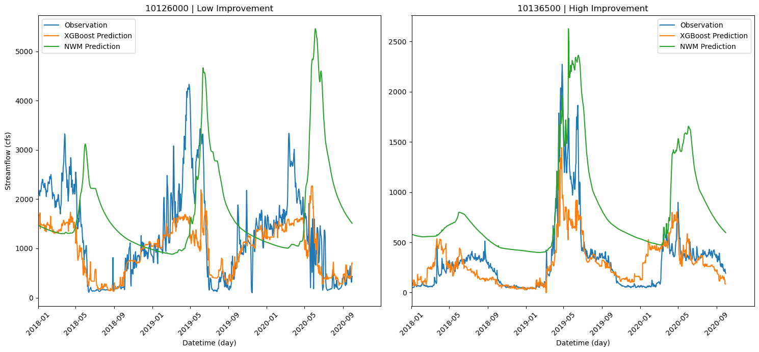
# The two stations with the highest and lowest improvement. 

two_list = ['10126000', '10136500']

two_list_name = ['Low', 'High']

# Initialize variables for the number of plots, columns, and rows based on the number of unique stations.
n_subplots = 2
n_cols = int(math.ceil(math.sqrt(n_subplots)))  # Calculate columns as the ceiling of the square root of number of subplots.
n_rows = int(math.ceil(n_subplots / n_cols))  # Calculate rows as the ceiling of the ratio of subplots to columns.
figsize = (15, 7)  # Set the figure size for the plot.
# Create a figure and a grid of subplots with the specified number of rows and columns.
fig, axes = plt.subplots(n_rows, n_cols, figsize=figsize)
axes = axes.flatten()  # Flatten the axes array for easier iteration.

# Iterate over each axis to plot data for each station.
for i, ax in enumerate(axes):
    if i < n_subplots:  # Check if the current index is less than the number of subplots to populate.

        # Get the observation data
        obs = data_test[data_test.station_id == two_list[i]][['datetime', 'flow_cfs', 'NWM_flow']].reset_index(drop=True)

        # Get the prediction data
        pred = final_output[two_list[i]].reset_index(drop=True)

        # Concat the two datastes
        eval_data = pd.concat([obs, pred], axis=1)

        # Set 'datetime' as the index for the DataFrame for plotting.
        temp_df_2 = eval_data.set_index('datetime')
        # Plot 'flow_cfs' on the primary y-axis.
        ax.plot(temp_df_2.index, temp_df_2['flow_cfs'], label='Observation')
        ax.plot(temp_df_2.index, temp_df_2['pred_cfs'], label='XGBoost Prediction')
        ax.plot(temp_df_2.index, temp_df_2['NWM_flow'], label='NWM Prediction')
        # Set x-axis limits from the minimum to maximum year of data.
        start_year = pd.to_datetime(f'{eval_data.datetime.dt.year.min()}-01-01')
        end_year = pd.to_datetime(f'{eval_data.datetime.dt.year.max()}-12-31')
        ax.set_xlim(start_year, end_year)
        # Get current x-tick labels and set their rotation for better visibility.
        labels = ax.get_xticklabels()
        ax.set_xticklabels(labels, rotation=45)

        # Set the title of the subplot to the station ID.
        ax.set_title(f'{two_list[i]} | {two_list_name[i]} Improvement')
        # Set the x-axis label for subplots in the last row.
        if i // n_cols == n_rows - 1:
            ax.set_xlabel('Datetime (day)')

        # Set the y-axis label for subplots in the first column.
        if i % n_cols == 0:
            ax.set_ylabel('Streamflow (cfs)')
        ax.legend()
    else:
        # Hide any unused axes.
        ax.axis('off')
        

# Adjust the layout to prevent overlapping elements.
plt.tight_layout()
# Uncomment the line below to save the figure to a file.
# plt.savefig(f'{save_path}scatter_annual_drought_number.png')
# Display the plot.
plt.show()

CPU times: user 328 ms, sys: 7.88 ms, total: 336 ms
Wall time: 335 ms

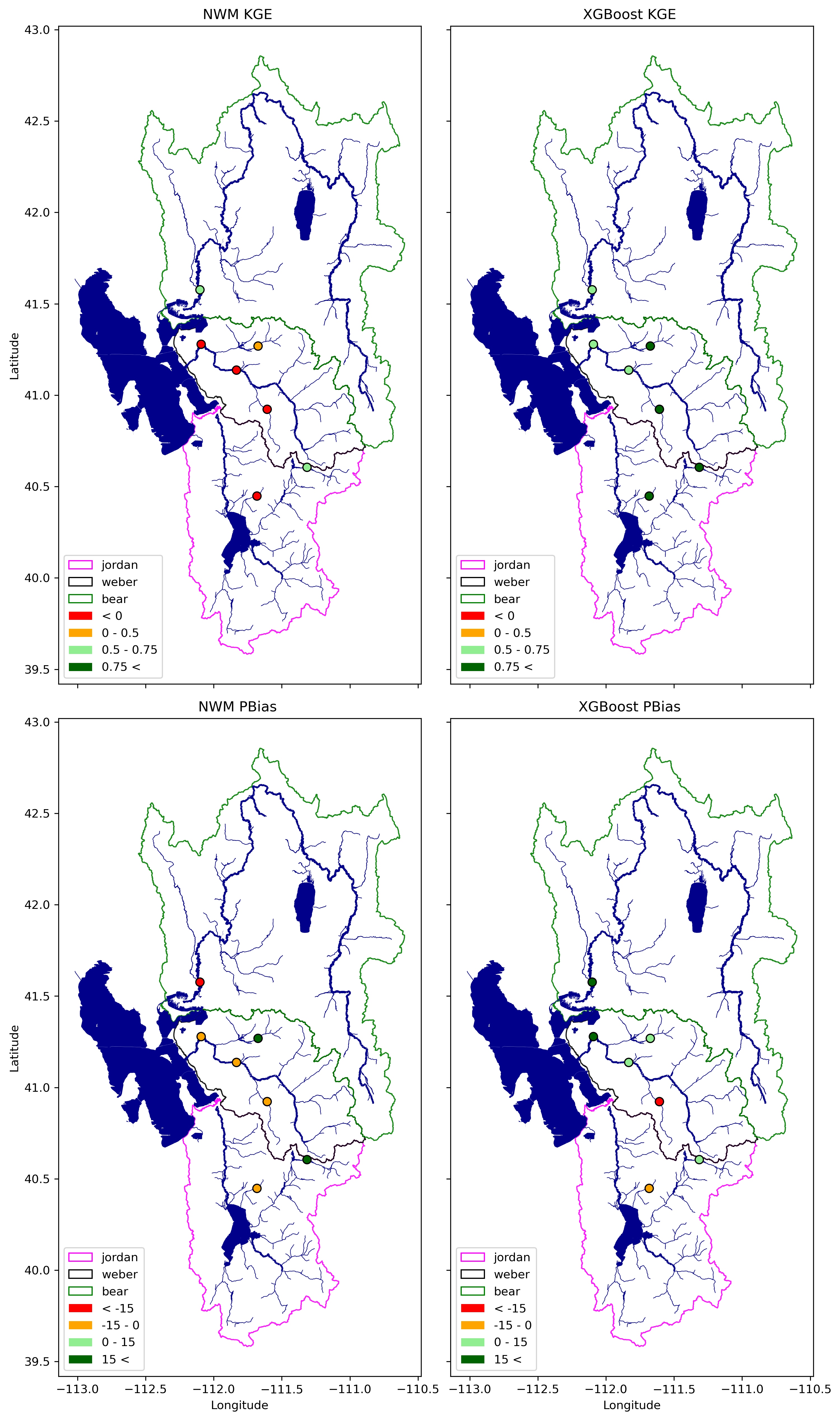
def categorize_kge(kge):
    if kge < 0:
        return 0
    elif 0 < kge <= 0.5:
        return 1
    elif 0.5 < kge <= 0.75:
        return 2
    elif 0.75 < kge :
        return 3

EvalDF_all_rf_all['NWM_KGE_cat'] = SupplyEvalDF_all_rf['NWM_KGE'].apply(categorize_kge)
EvalDF_all_rf_all['xgboost__KGE_cat'] = SupplyEvalDF_all_rf['xgboost__KGE'].apply(categorize_kge)

def categorize_pbias(pbias):
    if -15 < pbias < 0:
        return 0
    elif pbias < -15:
        return 1
    elif 0 < pbias < 15:
        return 2
    elif 15 < pbias :
        return 3    
EvalDF_all_rf_all['NWM_PBias_cat'] = SupplyEvalDF_all_rf['NWM_PBias'].apply(categorize_pbias)
EvalDF_all_rf_all['xgboost_PBias_cat'] = SupplyEvalDF_all_rf['xgboost_PBias'].apply(categorize_pbias)

%%time

# Specify the input path for your GeoPackage
geopackage_input = f'{input_path}all_shapes.gpkg'

file_list = ['jordan', 'weber', 'bear']

# Load and process the shapefiles from the GeoPackage
for file_name in file_list:
    gdf = gpd.read_file(geopackage_input, layer=file_name)

    # Merge all polygons into one
    merged_polygon = gdf.unary_union

    # Create a new GeoDataFrame
    merged_gdf = gpd.GeoDataFrame(geometry=[merged_polygon], crs=gdf.crs)

    # Save the merged polygon to a new layer in the GeoPackage
    merged_gdf.to_file(geopackage_input, layer=f"{file_name}_merged", driver="GPKG")

# Load the other layers from the GeoPackage
river_gdf_bear = gpd.read_file(geopackage_input, layer="river_bear")
river_gdf_jordan_weber = gpd.read_file(geopackage_input, layer="river_jordan_weber")
lake_gdf_jordan_weber = gpd.read_file(geopackage_input, layer="lake_jordan_weber")
lake_gdf_bear = gpd.read_file(geopackage_input, layer="lake_bear")

# Continue with the rest of your code unchanged...
from matplotlib.patches import Patch

year = ['NWM KGE', 'XGBoost KGE', 'NWM PBias', 'XGBoost PBias']
name = 'Severity'
variable = ['NWM_KGE_cat', 'xgboost__KGE_cat', 'NWM_PBias_cat', 'xgboost_PBias_cat']

fig, axes = plt.subplots(2, 2, figsize=(10, 17), dpi=300, sharey=True, sharex=True)
axes = axes.flatten()

for ax_index, ax in enumerate(axes):
    colors = ['fuchsia', 'black', 'green']

    if ax_index < 2:
        df_points = EvalDF_all_rf_all[['Lat', 'Long', 'NWM_KGE_cat', 'xgboost__KGE_cat']]
    elif ax_index >= 2:
        df_points = EvalDF_all_rf_all[['Lat', 'Long', 'NWM_PBias_cat', 'xgboost_PBias_cat']]

    for file_name, color_name in zip(file_list, colors):
        if color_name == 'fuchsia':
            my_zorder = 5
        else:
            my_zorder = 1

        merged_gdf = gpd.read_file(geopackage_input, layer=f"{file_name}_merged")

        merged_gdf.plot(ax=ax, alpha=0.9, facecolor='none', edgecolor=color_name, linewidth=1, label=file_name)
    
    lats = df_points['Lat']  # Example latitudes
    lons = df_points['Long']   # Example longitudes
    values = df_points[f'{variable[ax_index]}']  # Values associated with each point

    # Create GeoDataFrame from coordinates
    points_data = gpd.GeoDataFrame({'Latitude': lats, 'Longitude': lons, 'Value': values},
                                geometry=[Point(xy) for xy in zip(lons, lats)],
                                crs="EPSG:4326")  # Define the coordinate reference system

    subset = river_gdf_bear[river_gdf_bear['StreamLeve'] == 4]
    subset.plot(ax=ax, color='darkblue', linewidth=1.5, label=f'Stream Order', zorder=1)  # Multiply order by 2 for line width
    subset = river_gdf_bear[~(river_gdf_bear['StreamLeve'] == 4)]
    subset.plot(ax=ax, color='darkblue', linewidth=0.5, label=f'Stream Order', zorder=1)  # Multiply order by 2 for line width

    subset = river_gdf_jordan_weber[(river_gdf_jordan_weber['StreamLeve'] == 4) & ((river_gdf_jordan_weber['StreamOrde'] == 5) | (river_gdf_jordan_weber['StreamOrde'] == 6))]
    subset.plot(ax=ax, color='darkblue', linewidth=1.5, label=f'Stream Order', zorder=1)  # Multiply order by 2 for line width
    subset = river_gdf_jordan_weber[~((river_gdf_jordan_weber['StreamLeve'] == 4) & ((river_gdf_jordan_weber['StreamOrde'] == 5) | (river_gdf_jordan_weber['StreamOrde'] == 6)))]
    subset.plot(ax=ax, color='darkblue', linewidth=0.5, label=f'Stream Order', zorder=1)  # Multiply order by 2 for line width

    # Define colors for each value
    value_colors = {0: 'red', 1: 'orange', 2: 'lightgreen', 3: 'darkgreen'}

    # Plot the points GeoDataFrame with colors based on the 'Value'
    points_data.plot(ax=ax, marker='o', color=[value_colors[val] for val in points_data['Value']], markersize=50, label='Points', edgecolor='black', zorder=2)

    subset_lake_gdf_jordan_weber = lake_gdf_jordan_weber[(lake_gdf_jordan_weber['GNIS_Name'] != None) & (lake_gdf_jordan_weber['AreaSqKm'] >= 5) & ((lake_gdf_jordan_weber['FType'] == 390) | (lake_gdf_jordan_weber['FType'] == 436))]
    subset_lake_gdf_jordan_weber.plot(ax=ax, color='darkblue', linewidth=0.5, label=f'Stream Order', zorder=1)

    subset_lake_gdf_bear = lake_gdf_bear[(lake_gdf_bear['GNIS_Name'] != None) & (lake_gdf_bear['AreaSqKm'] >= 5) & ((lake_gdf_bear['FType'] == 390) | (lake_gdf_bear['FType'] == 436))]
    subset_lake_gdf_bear.plot(ax=ax, color='darkblue', linewidth=0.5, label=f'Stream Order', zorder=1)

    if ax_index < 2:
        colur_name = ['< 0', '0 - 0.5', '0.5 - 0.75', '0.75 <']
    if ax_index >= 2:
        colur_name = ['< -15', '-15 - 0', '0 - 15', '15 <']

    shapefile_handles = [Patch(facecolor='none', edgecolor=color, label=label) for color, label in zip(colors, file_list)]
    point_handles = [Patch(facecolor=color, edgecolor='none', label=f'{colur_name[val]}') for val, color in value_colors.items()]
    all_handles = shapefile_handles + point_handles

    ax.set_title(f'{year[ax_index]} ')
    if ax_index == 0 or ax_index == 2:
        ax.set_ylabel('Latitude')
    if ax_index >= 2:
        ax.set_xlabel('Longitude')

    ax.legend(handles=all_handles, loc='lower left')

plt.tight_layout()
plt.show()

CPU times: user 10.4 s, sys: 143 ms, total: 10.5 s
Wall time: 10.5 s