Model Development#
Machine Learning for Post-Processing NWM Data#
Authors: Savalan Naser Neisary (PhD Student, CIROH & The University of Alabama)
3. Setting Up the Codes and Notebook#
3.1. Access the GitHub Codes#
First we download the code files from the GitHub. In the terminal you should use the following command:
3.2. Import the Python Libraries#
Next we will import the libraries that we need.
!pip install hydroeval
Collecting hydroeval
  Downloading hydroeval-0.1.0-py3-none-any.whl.metadata (4.8 kB)
Requirement already satisfied: numpy in /home/runner/micromamba/envs/hackweek/lib/python3.12/site-packages (from hydroeval) (2.0.1)
Downloading hydroeval-0.1.0-py3-none-any.whl (22 kB)
Installing collected packages: hydroeval
Successfully installed hydroeval-0.1.0
# system packages
from datetime import datetime, date, timedelta
import pickle
import warnings
warnings.filterwarnings("ignore")
import platform
import time
from tqdm import tqdm
import os
import boto3
from botocore.client import Config
from botocore import UNSIGNED

# basic packages
import matplotlib.pyplot as plt
import numpy as np
import pandas as pd
import matplotlib.pyplot as plt
import matplotlib.dates as mdates
from matplotlib.patches import Patch
import math
from evaluation_table import EvalTable

# model packages
import xgboost as xgb
from sklearn.model_selection import GridSearchCV, train_test_split, RepeatedKFold, cross_val_score
from sklearn.metrics import mean_squared_error, mean_absolute_error, make_scorer
from sklearn.preprocessing import MinMaxScaler
import joblib
from shapely.geometry import Point
import geopandas as gpd
import pyproj

# Identify the path
home = os.getcwd()
parent_path = os.path.dirname(home)
input_path = f'{parent_path}/02.input/'
new_directory = os.path.join(parent_path, '03.output')
os.makedirs(new_directory, exist_ok=True)
output_path = f'{parent_path}/03.output/'
main_path = home
4. Data Preprocessing#
4.1. Overview of the USGS Stream Station#
The dataset that we will use provides the data for seven GSL watershed stations.
The dataset contains climate variables, such as precipitation and temperature, water infrastructure, storage percentage, and watershed characteristics, such as average area and elevation. You can see the location of the station and its watershed in the Figure below.
4.2. Load Dataset#
We will load the data from a parquet file and choose the required stations.
# List of station IDs that are of interest.
stations = ['10126000', '10130500', '10134500', '10136500', '10137500', '10141000', '10155000', '10164500', '10171000']

# Read a CSV file into a DataFrame and set the first column as the index.
df = df = pd.read_parquet(f'{input_path}final_input.parquet')

# Convert the station_id column to string data type.
df.station_id = df.station_id.astype(str)

# Convert the 'datetime' column to datetime objects.
df.datetime = pd.to_datetime(df.datetime)

# Filter the DataFrame to include only the rows where 'station_id' is in the 'stations' list.
df_modified = df[df['station_id'].isin(stations)]

# Select specific columns to create a new DataFrame.
dataset = df_modified[['station_id', 'datetime', 'Lat', 'Long', 'Drainage_area_mi2', 'Mean_Basin_Elev_ft',
       'Perc_Forest', 'Perc_Develop', 'Perc_Imperv', 'Perc_Herbace',
       'Perc_Slop_30', 'Mean_Ann_Precip_in', 's1',
       's2', 'storage', 'swe', 'NWM_flow', 'DOY','tempe(F)', 'precip(mm)', 'flow_cfs']]

# Extract a list of unique station IDs from the modified dataset.
station_list = dataset.station_id.unique()
4.3. Visualizing the Data#
The takeaway from data visualization is to gather information about data distribution, outliers, missing values, correlation between different variables, and time dependencies between variables.
Here, we will use boxplots, histograms, and combo bar and line plots to show outliers, distribution, and time dependencies in streamflow, precipitation, temperature, and SWE.
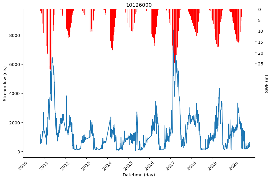
First, we will plot the time dependencies using bar and line plots for streamflow vs SWE.
%%time

figsize = (9, 6)  # Set the figure size for the plot.
fig, ax = plt.subplots(figsize=figsize)


# Extract data for the current station.
temp_df_1 = dataset[dataset.station_id == station_list[0]]
# Set 'datetime' as the index for the DataFrame for plotting.
temp_df_2 = temp_df_1.set_index('datetime')
# Plot 'flow_cfs' on the primary y-axis.
ax.plot(temp_df_2.index, temp_df_2['flow_cfs'])
# Set x-axis limits from the minimum to maximum year of data.
start_year = pd.to_datetime(f'{temp_df_1.datetime.dt.year.min()}-01-01')
end_year = pd.to_datetime(f'{temp_df_1.datetime.dt.year.max()}-12-31')
ax.set_xlim(start_year, end_year)
# Get current x-tick labels and set their rotation for better visibility.
labels = ax.get_xticklabels()
ax.set_xticklabels(labels, rotation=45)

# Create a secondary y-axis for Snow Water Equivalent (SWE).
ax2 = ax.twinx()
# Plot SWE as a bar graph on the secondary y-axis.
ax2.bar(temp_df_2.index, temp_df_2['swe'], label='Inverted', color='red')
# Set the y-axis limits for SWE, flipping the axis to make bars grow downward.
ax2.set_ylim(max(temp_df_2['swe']) + 40, 0)
# Set label for the secondary y-axis.
ax2.set_ylabel('SWE (in)')
# Define custom ticks for the secondary y-axis.
ax2.set_yticks(np.arange(0, max(temp_df_2['swe']), 5))

# Set the title of the subplot to the station ID.
ax.set_title(f'{station_list[0]}')
# Set the x-axis label for subplots in the last row.
ax.set_xlabel('Datetime (day)')

# Set the y-axis label for subplots in the first column.

ax.set_ylabel('Streamflow (cfs)')


# Adjust the layout to prevent overlapping elements.
plt.tight_layout()
# Uncomment the line below to save the figure to a file.
# plt.savefig(f'{save_path}scatter_annual_drought_number.png')
# Display the plot.
plt.show()
CPU times: user 2.36 s, sys: 67.3 ms, total: 2.43 s
Wall time: 2.41 s
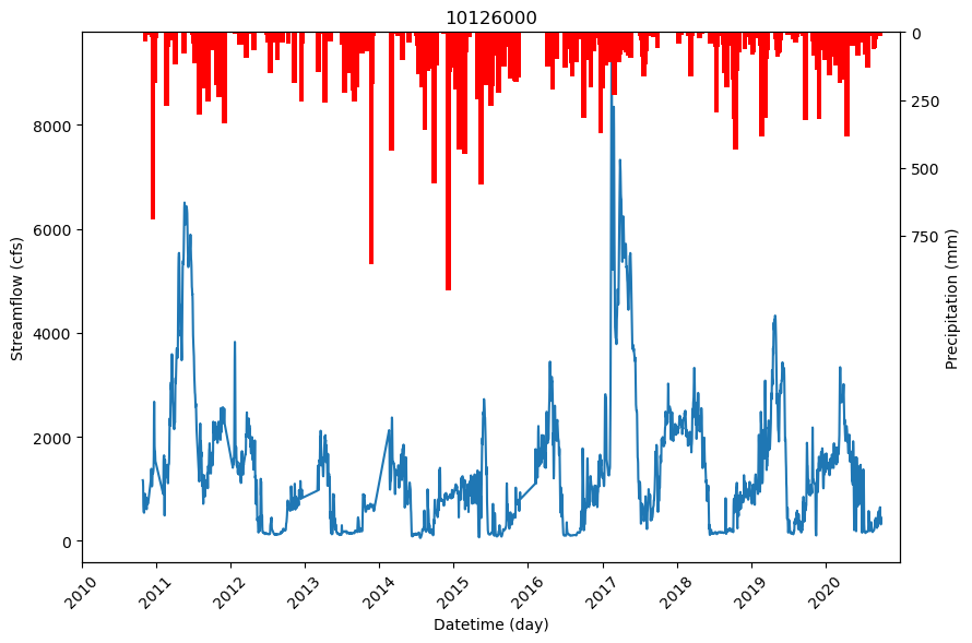
The next plot shows precipitation vs streamflow.
%%time

figsize = (9, 6)  # Set the figure size for the plot.
fig, ax = plt.subplots(figsize=figsize)


# Extract the data for the current station from the dataset.
temp_df_1 = dataset[dataset.station_id == station_list[0]]
# Set 'datetime' as the index for plotting.
temp_df_2 = temp_df_1.set_index('datetime')
# Plot the 'flow_cfs' data on the primary y-axis.
ax.plot(temp_df_2.index, temp_df_2['flow_cfs'])
# Set the x-axis limits from the first to the last year of data.
start_year = pd.to_datetime(f'{temp_df_1.datetime.dt.year.min()}-01-01')
end_year = pd.to_datetime(f'{temp_df_1.datetime.dt.year.max()}-12-31')
ax.set_xlim(start_year, end_year)
# Rotate x-axis labels for better readability.
labels = ax.get_xticklabels()
ax.set_xticklabels(labels, rotation=45)

# Create a second y-axis for the precipitation data.
ax2 = ax.twinx()
# Plot the 'precip(mm)' data as a bar graph on the secondary y-axis.
ax2.bar(temp_df_2.index, temp_df_2['precip(mm)'], label='Inverted', color='red', width=25)
# Set the y-axis limits for precipitation, flipping the axis to make bars grow downward.
ax2.set_ylim(max(temp_df_2['precip(mm)']) + 1000, 0)
# Set the label for the secondary y-axis.
ax2.set_ylabel('Precipitation (mm)')
# Define custom ticks for the secondary y-axis.
ax2.set_yticks(np.arange(0, max(temp_df_2['precip(mm)']), 250))

# Set the title of the subplot to the station ID.
ax.set_title(f'{station_list[0]}')
# Set the x-axis label for subplots in the last row.

ax.set_xlabel('Datetime (day)')

# Set the y-axis label for subplots in the first column.

ax.set_ylabel('Streamflow (cfs)')


# Adjust the layout to prevent overlapping elements.
plt.tight_layout()
# Uncomment the line below to save the figure to a file.
# plt.savefig(f'{save_path}scatter_annual_drought_number.png')
# Display the plot.
plt.show()
CPU times: user 2.47 s, sys: 27.6 ms, total: 2.5 s
Wall time: 2.48 s
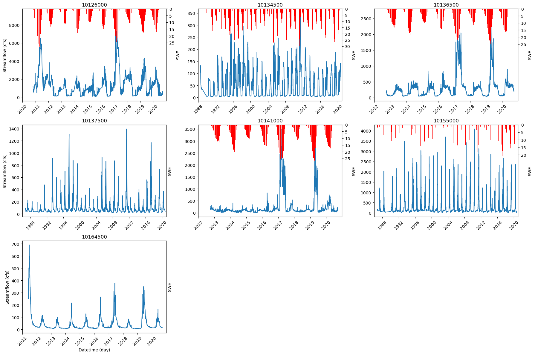
Now we will plot all the stations.
%%time
# Initialize variables for the number of plots, columns, and rows based on the number of unique stations.
n_subplots = len(station_list)
n_cols = int(math.ceil(math.sqrt(n_subplots)))  # Calculate columns as the ceiling of the square root of number of subplots.
n_rows = int(math.ceil(n_subplots / n_cols))  # Calculate rows as the ceiling of the ratio of subplots to columns.
figsize = (18, 12)  # Set the figure size for the plot.
# Create a figure and a grid of subplots with the specified number of rows and columns.
fig, axes = plt.subplots(n_rows, n_cols, figsize=figsize)
axes = axes.flatten()  # Flatten the axes array for easier iteration.

# Iterate over each axis to plot data for each station.
for i, ax in enumerate(axes):
    if i < n_subplots:  # Check if the current index is less than the number of subplots to populate.
        # Extract data for the current station.
        temp_df_1 = dataset[dataset.station_id == station_list[i]]
        # Set 'datetime' as the index for the DataFrame for plotting.
        temp_df_2 = temp_df_1.set_index('datetime')
        # Plot 'flow_cfs' on the primary y-axis.
        ax.plot(temp_df_2.index, temp_df_2['flow_cfs'])
        # Set x-axis limits from the minimum to maximum year of data.
        start_year = pd.to_datetime(f'{temp_df_1.datetime.dt.year.min()}-01-01')
        end_year = pd.to_datetime(f'{temp_df_1.datetime.dt.year.max()}-12-31')
        ax.set_xlim(start_year, end_year)
        # Get current x-tick labels and set their rotation for better visibility.
        labels = ax.get_xticklabels()
        ax.set_xticklabels(labels, rotation=45)

        # Create a secondary y-axis for Snow Water Equivalent (SWE).
        ax2 = ax.twinx()
        # Plot SWE as a bar graph on the secondary y-axis.
        ax2.bar(temp_df_2.index, temp_df_2['swe'], label='Inverted', color='red')
        # Set the y-axis limits for SWE, flipping the axis to make bars grow downward.
        ax2.set_ylim(max(temp_df_2['swe']) + 40, 0)
        # Set label for the secondary y-axis.
        ax2.set_ylabel('SWE')
        # Define custom ticks for the secondary y-axis.
        ax2.set_yticks(np.arange(0, max(temp_df_2['swe']), 5))

        # Set the title of the subplot to the station ID.
        ax.set_title(f'{station_list[i]}')
        # Set the x-axis label for subplots in the last row.
        if i // n_cols == n_rows - 1:
            ax.set_xlabel('Datetime (day)')

        # Set the y-axis label for subplots in the first column.
        if i % n_cols == 0:
            ax.set_ylabel('Streamflow (cfs)')
    else:
        # Hide any unused axes.
        ax.axis('off')

# Adjust the layout to prevent overlapping elements.
plt.tight_layout()
# Uncomment the line below to save the figure to a file.
# plt.savefig(f'{save_path}scatter_annual_drought_number.png')
# Display the plot.
plt.show()
CPU times: user 31.5 s, sys: 424 ms, total: 31.9 s
Wall time: 31.8 s
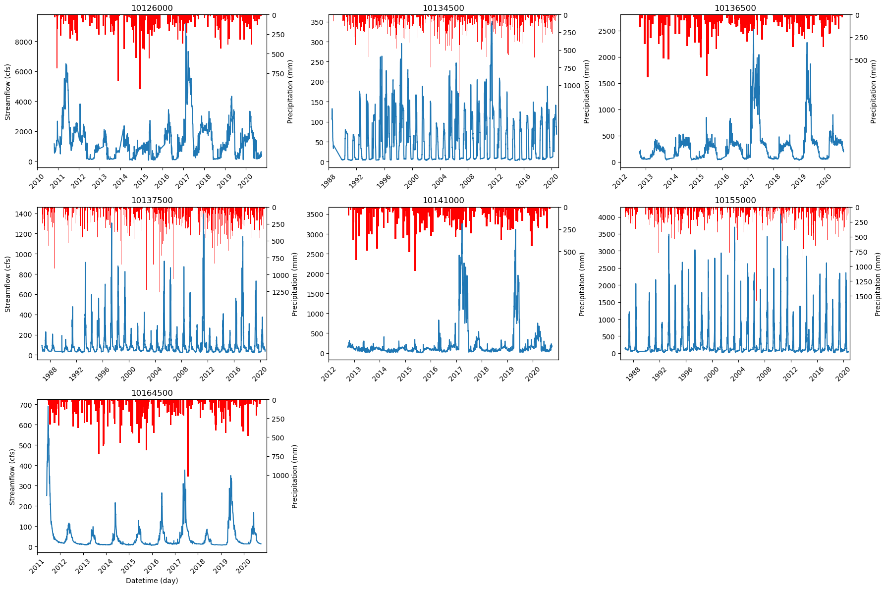
%%time
# Calculate the number of subplots needed based on the number of unique stations.
n_subplots = len(station_list)
# Determine the number of columns in the subplot grid by taking the ceiling of the square root of 'n_subplots'.
n_cols = int(math.ceil(math.sqrt(n_subplots)))
# Determine the number of rows in the subplot grid by dividing 'n_subplots' by 'n_cols' and taking the ceiling of that.
n_rows = int(math.ceil(n_subplots / n_cols))
# Set the figure size for the subplots.
figsize = (18, 12)
# Create a grid of subplots with specified number of rows and columns and figure size.
fig, axes = plt.subplots(n_rows, n_cols, figsize=figsize)
# Flatten the axes array for easier iteration.
axes = axes.flatten()

# Iterate over the axes to plot the data for each station.
for i, ax in enumerate(axes):
    if i < n_subplots:
        # Extract the data for the current station from the dataset.
        temp_df_1 = dataset[dataset.station_id == station_list[i]]
        # Set 'datetime' as the index for plotting.
        temp_df_2 = temp_df_1.set_index('datetime')
        # Plot the 'flow_cfs' data on the primary y-axis.
        ax.plot(temp_df_2.index, temp_df_2['flow_cfs'])
        # Set the x-axis limits from the first to the last year of data.
        start_year = pd.to_datetime(f'{temp_df_1.datetime.dt.year.min()}-01-01')
        end_year = pd.to_datetime(f'{temp_df_1.datetime.dt.year.max()}-12-31')
        ax.set_xlim(start_year, end_year)
        # Rotate x-axis labels for better readability.
        labels = ax.get_xticklabels()
        ax.set_xticklabels(labels, rotation=45)

        # Create a second y-axis for the precipitation data.
        ax2 = ax.twinx()
        # Plot the 'precip(mm)' data as a bar graph on the secondary y-axis.
        ax2.bar(temp_df_2.index, temp_df_2['precip(mm)'], label='Inverted', color='red', width=25)
        # Set the y-axis limits for precipitation, flipping the axis to make bars grow downward.
        ax2.set_ylim(max(temp_df_2['precip(mm)']) + 1000, 0)
        # Set the label for the secondary y-axis.
        ax2.set_ylabel('Precipitation (mm)')
        # Define custom ticks for the secondary y-axis.
        ax2.set_yticks(np.arange(0, max(temp_df_2['precip(mm)']), 250))

        # Set the title of the subplot to the station ID.
        ax.set_title(f'{station_list[i]}')
        # Set the x-axis label for subplots in the last row.
        if i // n_cols == n_rows - 1:
            ax.set_xlabel('Datetime (day)')

        # Set the y-axis label for subplots in the first column.
        if i % n_cols == 0:
            ax.set_ylabel('Streamflow (cfs)')
    else:
        # Hide any unused axes.
        ax.axis('off')

# Adjust layout to prevent overlapping elements.
plt.tight_layout()
# Uncomment the line below to save the figure to a file.
# plt.savefig(f'{save_path}scatter_annual_drought_number.png')
# Display the plot.
plt.show()
CPU times: user 31.8 s, sys: 555 ms, total: 32.3 s
Wall time: 32.1 s
4.4. Splitting the Data#
We split 80 percent of the data for training and the rest for testing the model.
# Create empty DataFrames for training and testing datasets.
data_train = pd.DataFrame()
data_test = pd.DataFrame()

# Loop through each station name in the list of station IDs.
for station_name in station_list:
    # Extract data for the current station and reset the index.
    temp_df_1 = dataset[dataset.station_id == station_name].reset_index(drop=True)

    # Determine the maximum and minimum years in the dataset for the current station.
    end_year = temp_df_1.datetime.dt.year.max()
    start_year = temp_df_1.datetime.dt.year.min()

    # Calculate the duration in years between the earliest and latest data points.
    duration = end_year - start_year

    # Calculate the division year to split training and testing data (80% for training).
    division_year = start_year + int(duration * 0.8)

    # Select data from the start year up to the division year for training, reset the index, and append to the training DataFrame.
    data_train = pd.concat((data_train.reset_index(drop=True), temp_df_1[temp_df_1.datetime < f'{division_year}-01-01'].reset_index(drop=True)), axis=0).reset_index(drop=True)

    # Select data from the division year onward for testing, reset the index, and append to the testing DataFrame.
    data_test = pd.concat((data_test.reset_index(drop=True), temp_df_1[temp_df_1.datetime >= f'{division_year}-01-01'].reset_index(drop=True)), axis=0).reset_index(drop=True)
5. Model Development#
5.1. Defining the XGBoost Model#
As mentioned, we will use XGBoost in our tutorial, and we will use the dmlc XGBoost package. Understanding and tuning the model parameters is critical in any ML model development since it will affect the final model performance. The XGBoost model has different parameters, and here, we will work on the three most important parameters of XGBoost:
max_depthThis parameter determines the maximum depth of each tree. This setting controls the complexity of the tree by restricting the number of levels or splits within it. Increasing the max_depth can help capture more complex patterns in the data, but it can also lead to overfitting, where the model becomes too specialized in the training data and performs poorly on new data. On the other hand, reducing the max_depth can help prevent overfitting, but it can also result in underfitting, where the model misses relevant patterns.n_estimatorsIt determines the number of trees in the ensemble and controls how many boosting rounds the algorithm should perform. Boosting rounds add new trees that attempt to correct errors from previous rounds, leading to improved performance up to a point. However, too many trees can result in overfitting, where the model performs well on training data but poorly on unseen data. It also increases the running time of the model.etaIt controls the step size used to update the weights of the trees during training and determines how much each new tree contributes to the overall model. A smaller eta value can make the model more robust to overfitting by slowing the learning process. However, more boosting rounds (n_estimators) may be required to achieve good performance. Conversely, a larger eta value allows the model to learn faster but increases the risk of overfitting.
We will call the XGBRegressor() model and specify its parameters.
To make the process faster for this part we only use one station.
Let’s start investigating different parameters and find out the best possible values!!!!!!!!!!!!!!!!!
def evaluate_model(params, X_train, y_train):
    # Create an XGBoost regressor model with the provided parameters.
    model = xgb.XGBRegressor(**params)

    # Set up cross-validation configuration with 10 splits and 3 repeats, and a fixed random state for reproducibility.
    cv = RepeatedKFold(n_splits=10, n_repeats=3, random_state=1)

    # Perform cross-validation to evaluate the model using the negative mean absolute error as the scoring method.
    # 'n_jobs=-1' enables using all CPU cores for parallel computation.
    scores = cross_val_score(model, X_train, y_train, scoring='neg_mean_absolute_error', cv=cv, n_jobs=-1)

    # Return the scores from the cross-validation.
    return scores
# Define the station ID to be used.
station_name = '10126000'
# Select and reset the index of feature columns from the training data where station ID matches.
x_train = data_train[data_train.station_id == station_name].iloc[:, 2:-1].reset_index(drop=True)
# Select and reset the index of the target column from the training data where station ID matches.
y_train = data_train[data_train.station_id == station_name].iloc[:, -1].reset_index(drop=True)

# Define the initial parameters for the XGBoost model.
# n_estimators => 100, 2000
# max_depth => 3, 10
# eta => 0.01, 0.1

params = {
    'n_estimators': 200,
    'max_depth': 5,
    'eta': 0.1,
}

# Evaluate the model with initial parameters and calculate the mean of absolute scores.
current_score = abs(evaluate_model(params, x_train, y_train).mean())
print(f"Initial score (cfs): {current_score} with params: {params}")

# Initialize the interactive tuning loop.
continue_tuning = True
while continue_tuning:
    # Prompt the user if they want to continue tuning.
    print('=====================================================================================')
    change = "n" # to interact with this notebook using input(), comment out this line, and uncomment the line below
    # change = input("Do you want to change any variable? (y/n): ")
    if change.lower() == 'y':
        # Ask which parameter to change.
        variable = input("Which variable number? (n_estimators(1)/max_depth(2)/eta(3)):")
        # Map user input to the corresponding parameter.
        if variable == '1':
            variable = 'n_estimators'
        elif variable == '2':
            variable = 'max_depth'
        elif variable == '3':
            variable = 'eta'
        else:
            print('Error: Wrong Number')
            break

        # Prompt for the new value and validate the type.
        value = input(f"Enter the new value for {variable} (previous value {params[variable]}): ")
        if variable == 'n_estimators' or variable == 'max_depth':
            value = int(value)
        else:
            value = float(value)

        # Update parameter and re-evaluate the model.
        old_param = params[variable]
        params[variable] = value
        new_score = evaluate_model(params, x_train, y_train)
        print('**********************************************')
        print('Previous Mean Score (cfs): %.3f (Previous Score SD: %.3f)' % (abs(current_score.mean()), current_score.std()))
        print('New Mean Score (cfs): %.3f (New Score SD: %.3f)' % (abs(new_score.mean()), new_score.std()))
        print('**********************************************')
        current_score = new_score

        # Prompt if the new parameter setting should be kept.
        keep_answer = input(f"Do you want to keep the new variable?(y/n): ")
        if keep_answer == 'n':
            params[variable] = old_param
    else:
        # Exit tuning loop.
        continue_tuning = False
        print(f"Finished tuning ====================> Final parameters: {params}.")
Initial score (cfs): 152.80558477080083 with params: {'n_estimators': 200, 'max_depth': 5, 'eta': 0.1}
=====================================================================================
Finished tuning ====================> Final parameters: {'n_estimators': 200, 'max_depth': 5, 'eta': 0.1}.
!!!! Don’t forget to train and save your model after tuning the hyperparameters as a Pickle file.
# Instantiate an XGBoost regressor model with the specified parameters.
xgboost_model = xgb.XGBRegressor(**params)

# Fit the model using the training dataset.
xgboost_model.fit(x_train, y_train)

# Save the trained model to a file using the pickle library for later use.
# 'save_path' should be defined earlier in your script and point to a directory where you have write permissions.
pickle.dump(xgboost_model, open(f'{output_path}best_manuall_model.pkl', "wb"))
data_train.to_pickle(f"{output_path}train_dataset.pkl")
data_test.to_pickle(f"{output_path}test_dataset.pkl")